Gostaria de compartilhar uma prática simples mas, de grande valia na rotina de caracterização de reservatórios óleo e gás. É corriqueira a realização de algumas etapas na caracterização desses reservatórios a partir de dados sísmicos e de logs de poços. Porém, esses produtos são amparados na informação de dados de poços. Essa informação é o que chamamos de dado hard é a informação mais fidedigna a respeito de uma litologia. Para que a os estudos de reservatório tenha sucesso é, fundamental garantir uma boa qualidade de seus inputs. É aí que entra a aplicação do conceito de outliers. Muitas vezes os perfis de poços carregam valores espúrios oriundos da coleta por isso tão importante tratá-los. Aqui fiz uma aplicação simples que se faz importante na petrofísica, geologia e geofísica mas que podemos extender para inúmeros casos na rotina de trabalho. Vou mostrar como carregar perfis no formato las e construir essa análise de outliers na forma gráfica de boxplots. Para tal, será usada a linguagem Python. Os dados de input foram dados open source do Campo de Otway na Austrália.
Instalação de Bibliotecas
import pandas as pd
import numpy as np
import seaborn as sns
import matplotlib.pyplot as plt
import lasio
%matplotlib inline

print("installed")
installed
LISTA PARA CARREGAMENTO DOS POCOS
Input_path="/home/ ....  /OtwayBasin/*.las"
import glob
my_list=[glob.glob(Input_path)]
print("Número de poços carregados",len(my_list[0])) #>>> para exibir o numero de pocos carregados
Número de poços carregados 78
CARREGAMENDO COM O LASIO
#Todos os pocos carregados com pseudonome "P"
for i in range(len(my_list[0])):
    globals()["P" + str(i)]=lasio.read(my_list[0][i]).df()
    globals()["P" + str(i)]= globals()["P" + str(i)].reindex(sorted(globals()["P" + str(i)].columns), axis=1)
    i=i+1
TESTE
#vamos imputar os dados faltantes TESTE
lista_colunas=['CALI','DRHO','DT','GR','NPHI','RDEP','RHOB','RMED','RMIC','SP','WELL']
print(len(lista_colunas))
print(len(globals()["P" + str(1)].columns))
print(list(set(lista_colunas) -set(P1.columns)))
P1.columns
11
13
['WELL']


Index(['CALI', 'DRHO', 'DT', 'GR', 'MINV', 'MNOR', 'NPHI', 'PEF', 'RDEP',
       'RHOB', 'RMED', 'RMIC', 'SP'],
      dtype='object')
CRIAÇÃO DE LOG FALTANTE COM NAN
for i in range(len(my_list[0])):
    if(list(set(lista_colunas) -set(globals()["P" + str(i)].columns)) != []):
        diff_list = list(set(lista_colunas) -set(globals()["P" + str(i)].columns))
        print(i,diff_list)
        for j in range(len(diff_list)): #adiciona cada coluna por vez de acordo c a diff_list
            globals()["P" + str(i)][diff_list[j]] = pd.Series(np.nan, index=globals()["P" + str(i)].index)

        j=j+1
    #reordena por ordem alfabética cada dataframe
    globals()["P" + str(i)]= globals()["P" + str(i)].reindex(sorted(globals()["P" + str(i)].columns), axis=1)
    i=i+1
    print(i," ____")
0 ['WELL', 'NPHI', 'DRHO', 'RHOB']
1  ____
1 ['WELL']
2  ____
2 ['WELL']
3  ____
3 ['WELL']
4  ____
4 ['WELL']
5  ____
5 ['WELL']
6  ____
6 ['WELL']
7  ____
7 ['WELL']
8  ____
8 ['WELL', 'RMED', 'SP', 'RDEP']
9  ____
9 ['WELL', 'NPHI', 'DRHO', 'RHOB']
10  ____
10 ['WELL']
11  ____
11 ['WELL']
12  ____
12 ['WELL']
13  ____
13 ['WELL', 'CALI', 'RMIC', 'RHOB', 'DRHO', 'NPHI']
14  ____
14 ['WELL']
15  ____
15 ['WELL']
16  ____
16 ['WELL', 'DT', 'CALI', 'RMIC', 'RHOB', 'DRHO', 'NPHI']
17  ____
17 ['WELL']
18  ____
18 ['WELL', 'RMIC', 'RHOB', 'DRHO', 'NPHI']
19  ____
19 ['WELL']
20  ____
20 ['WELL']
21  ____
21 ['WELL']
22  ____
22 ['WELL']
23  ____
23 ['WELL']
24  ____
24 ['WELL', 'DT', 'RMIC', 'RHOB', 'GR', 'DRHO', 'NPHI']
25  ____
25 ['WELL', 'RMIC', 'RHOB', 'DRHO', 'NPHI']
26  ____
26 ['WELL']
27  ____
27 ['WELL']
28  ____
28 ['WELL', 'RMIC', 'NPHI']
29  ____
29 ['WELL', 'SP', 'RHOB', 'DRHO', 'NPHI']
30  ____
30 ['WELL']
31  ____
31 ['WELL']
32  ____
32 ['WELL']
33  ____
33 ['WELL']
34  ____
34 ['WELL', 'RMIC', 'RHOB', 'DRHO', 'NPHI']
35  ____
35 ['WELL']
36  ____
36 ['WELL', 'DT', 'RMIC', 'RHOB', 'GR', 'DRHO', 'NPHI']
37  ____
37 ['WELL', 'RMED', 'SP', 'RDEP']
38  ____
38 ['WELL']
39  ____
39 ['WELL']
40  ____
40 ['WELL']
41  ____
41 ['WELL']
42  ____
42 ['WELL']
43  ____
43 ['WELL']
44  ____
44 ['WELL']
45  ____
45 ['WELL']
46  ____
46 ['WELL', 'RMIC', 'RHOB', 'DRHO', 'NPHI']
47  ____
47 ['WELL']
48  ____
48 ['WELL', 'NPHI', 'DRHO', 'RHOB']
49  ____
49 ['WELL']
50  ____
50 ['WELL']
51  ____
51 ['WELL']
52  ____
52 ['WELL', 'NPHI', 'DRHO', 'RHOB']
53  ____
53 ['WELL', 'RMIC']
54  ____
54 ['WELL']
55  ____
55 ['WELL']
56  ____
56 ['WELL']
57  ____
57 ['WELL', 'DT', 'CALI', 'RMIC', 'RHOB', 'DRHO', 'NPHI']
58  ____
58 ['WELL', 'SP']
59  ____
59 ['WELL', 'RMIC', 'NPHI']
60  ____
60 ['WELL', 'RMIC']
61  ____
61 ['WELL', 'RMIC', 'RHOB', 'DRHO', 'NPHI']
62  ____
62 ['WELL']
63  ____
63 ['WELL', 'CALI', 'RMIC', 'RHOB', 'DRHO', 'NPHI']
64  ____
64 ['WELL', 'RMIC', 'RHOB', 'DRHO', 'NPHI']
65  ____
65 ['WELL']
66  ____
66 ['WELL']
67  ____
67 ['WELL']
68  ____
68 ['WELL']
69  ____
69 ['WELL', 'NPHI', 'DRHO', 'RHOB']
70  ____
70 ['WELL', 'RMIC', 'NPHI']
71  ____
71 ['WELL', 'RMIC']
72  ____
72 ['WELL']
73  ____
73 ['WELL', 'DT', 'RMED', 'SP', 'CALI', 'RMIC', 'RHOB', 'GR', 'DRHO', 'NPHI']
74  ____
74 ['WELL']
75  ____
75 ['WELL']
76  ____
76 ['WELL', 'RMIC', 'RHOB', 'DRHO', 'NPHI']
77  ____
77 ['WELL']
78  ____
P29
| CALI | DRHO | DT | GR | NPHI | RDEP | RHOB | RMED | RMIC | SP | WELL | |
|---|---|---|---|---|---|---|---|---|---|---|---|
| DEPTH | |||||||||||
| 0.0000 | NaN | NaN | NaN | NaN | NaN | NaN | NaN | NaN | NaN | NaN | NaN |
| 0.1524 | NaN | NaN | NaN | NaN | NaN | NaN | NaN | NaN | NaN | NaN | NaN |
| 0.3048 | NaN | NaN | NaN | NaN | NaN | NaN | NaN | NaN | NaN | NaN | NaN |
| 0.4572 | NaN | NaN | NaN | NaN | NaN | NaN | NaN | NaN | NaN | NaN | NaN |
| 0.6096 | NaN | NaN | NaN | NaN | NaN | NaN | NaN | NaN | NaN | NaN | NaN |
| ... | ... | ... | ... | ... | ... | ... | ... | ... | ... | ... | ... |
| 1094.5368 | NaN | NaN | NaN | NaN | NaN | NaN | NaN | NaN | NaN | NaN | NaN |
| 1094.6892 | NaN | NaN | NaN | NaN | NaN | NaN | NaN | NaN | NaN | NaN | NaN |
| 1094.8416 | NaN | NaN | NaN | NaN | NaN | NaN | NaN | NaN | NaN | NaN | NaN |
| 1094.9940 | NaN | NaN | NaN | NaN | NaN | NaN | NaN | NaN | NaN | NaN | NaN |
| 1095.1464 | NaN | NaN | NaN | NaN | NaN | NaN | NaN | NaN | NaN | NaN | NaN |
7187 rows × 11 columns
JUNÇÃO DE TODOS OS POÇOS EM UNICO ARQUIVO
#todos os pocos com os perfis


lista_pocos=['P1','P9','P10','P14','P17','P19','P25','P26','P30','P35','P37','P38','P47','P49','P53','P58','P62','P64','P65','P70','P74','P77']
all_wells=pd.DataFrame()
all_wells=P1
#for i in range(len(my_list[0])):
for i in range(len(lista_pocos)):
    all_wells=all_wells.append((globals()[str(lista_pocos[i])]))
    i=i+1
all_wells.describe()
| CALI | DRHO | DT | GR | MINV | MNOR | NPHI | PEF | RDEP | RHOB | RMED | RMIC | SP | WELL | DTS | NEUT | |
|---|---|---|---|---|---|---|---|---|---|---|---|---|---|---|---|---|
| count | 275651.000000 | 164388.000000 | 290362.000000 | 373447.000000 | 116505.000000 | 116505.000000 | 160307.000000 | 145218.000000 | 256111.000000 | 164471.000000 | 260299.000000 | 199014.000000 | 249079.000000 | 0.0 | 20004.000000 | 2370.000000 |
| mean | 9.410099 | 0.071992 | 96.720829 | 80.824487 | 3.389594 | 2.661659 | 0.259453 | 3.026118 | 22.292091 | 2.358424 | 18.930929 | 41.241388 | 37.444625 | NaN | 143.465757 | 1330.494785 |
| std | 1.895997 | 0.096493 | 24.467956 | 36.358582 | 8.224229 | 5.355036 | 0.106553 | 0.914562 | 820.143139 | 0.191193 | 715.466800 | 953.697102 | 85.795078 | NaN | 20.631918 | 265.019184 |
| min | -3.680000 | -2.086000 | -19.000000 | 0.000000 | 0.025000 | -0.342800 | -0.045500 | 0.000000 | 0.000000 | 0.000000 | 0.000000 | 0.000000 | -135.375000 | NaN | 76.053900 | 487.062400 |
| 25% | 8.497100 | 0.000000 | 79.400000 | 51.000000 | 0.419900 | 0.482600 | 0.191900 | 2.539100 | 2.164550 | 2.249700 | 2.092500 | 1.110500 | -21.822800 | NaN | 128.955625 | 1260.929225 |
| 50% | 8.850000 | 0.027300 | 90.150000 | 85.688600 | 1.114800 | 1.004700 | 0.264300 | 2.955100 | 4.375200 | 2.392000 | 4.720600 | 2.085100 | 10.300000 | NaN | 146.815150 | 1369.418600 |
| 75% | 9.750000 | 0.127700 | 110.800000 | 109.683500 | 2.765400 | 1.977300 | 0.334500 | 3.294000 | 8.752550 | 2.494300 | 9.607700 | 4.149500 | 74.687800 | NaN | 158.783100 | 1471.396100 |
| max | 40.620000 | 3.154600 | 1183.000000 | 803.201600 | 374.234400 | 95.289100 | 3.276700 | 10.258700 | 60000.000000 | 3.239900 | 60000.000000 | 24945.929700 | 4528.000000 | NaN | 190.523700 | 2088.022500 |
Missing values
Em dados do tipo LAS file a ausência de dado (medição) é representado pelo valor -99999.0 é o nosso null value. Onde houve a ausência desses dados a função isna retornará com o boleano True na posição faltante ou False caso contrário. E para contabilizar esses valores faltante será feita uma somatória com a função sum descrito abaixo:
#Counting all Nan values(percentage) in each well log
Tot_nan=all_wells.isna().sum()
Tot_not_nan=all_wells.count()#essa variável nao leva em consideração numero de nan

100*Tot_nan/(Tot_nan+Tot_not_nan)
#in percentage : missing values
CALI     27.042099
DRHO     56.490623
DT       23.148467
GR        1.157953
MINV     69.164051
MNOR     69.164051
NPHI     57.570761
PEF      61.564440
RDEP     32.213847
RHOB     56.468655
RMED     31.105388
RMIC     47.325989
SP       34.075041
WELL    100.000000
DTS      94.705443
NEUT     99.372720
dtype: float64
PARA O EXERCICIO VOU SELECIONAR SOMENTE NPHI, GR, RHOB,DT
all_wells_D=all_wells.drop(['CALI','RDEP','RMED','RMIC','SP','DRHO','PEF','NEUT','MINV','MNOR','WELL'],axis=1)
Calculando o número de Nan values em cada perfil
O proximo passo será a remoção das linhas cujo dado esteja faltante em algun log selecionado. E em seguida calcular o quanto se eliminou em termos de linhas em relação ao dado original.
all_wells_dropped = all_wells_D.dropna(axis=0, how='any')
print("ANTES DO DROPNA",all_wells.shape)
print("DEPOIS DO DROPNA",all_wells_dropped.shape)
print("  ")
A=(145975*11/306849*15)
print("REDUÇÃO DO DADO EM %.3f"% A)
ANTES DO DROPNA (377822, 16)
DEPOIS DO DROPNA (13892, 5)

REDUÇÃO DO DADO EM 78.494
Statistics
O comando describe é muito útil para observar a estatística do dado.
all_wells_dropped.head()
| DT | GR | NPHI | RHOB | DTS | |
|---|---|---|---|---|---|
| DEPTH | |||||
| 2898.8004 | 68.0511 | 97.7741 | 0.2354 | 2.0982 | 158.2822 |
| 2898.9528 | 69.5735 | 95.8630 | 0.2674 | 2.1121 | 158.2287 |
| 2899.1052 | 71.8478 | 97.5757 | 0.2990 | 2.1082 | 160.2277 |
| 2899.2576 | 75.6225 | 89.2717 | 0.2782 | 2.0961 | 164.1069 |
| 2899.4100 | 79.0742 | 90.0361 | 0.2613 | 2.0752 | 163.9499 |
Produzindo o Boxplot com outliers
import seaborn as sns
all_wells_dropped.describe()
| DT | GR | NPHI | RHOB | DTS | |
|---|---|---|---|---|---|
| count | 13892.000000 | 13892.000000 | 13892.000000 | 13892.000000 | 13892.000000 |
| mean | 77.362332 | 93.121544 | 0.165715 | 2.432747 | 140.459897 |
| std | 9.475476 | 41.846689 | 0.105444 | 0.153735 | 18.057316 |
| min | 0.000000 | 0.000000 | -0.005600 | 0.000000 | 85.413400 |
| 25% | 69.967775 | 64.501750 | 0.078000 | 2.383200 | 126.218950 |
| 50% | 76.292350 | 87.457550 | 0.144900 | 2.466200 | 141.008850 |
| 75% | 84.341425 | 117.480675 | 0.249400 | 2.523100 | 153.344200 |
| max | 119.328400 | 803.201600 | 0.534300 | 3.008400 | 190.523700 |
criando coluna com poços
df1=pd.DataFrame({'VALUE':all_wells_dropped['DT']})
df2=pd.DataFrame({'VALUE':all_wells_dropped['GR']})
df3=pd.DataFrame({'VALUE':all_wells_dropped['NPHI']})
df4=pd.DataFrame({'VALUE':all_wells_dropped['RHOB']})
df1['LOG'] = 'DT'
df2['LOG'] = 'GR'
df3['LOG'] = 'NPHI'
df4['LOG'] = 'RHOB'
Vamos aos plots
É importante entender que durante o processo de perfilagem podem aparecer dados espúrios por isso vamos olhar a distribuição de cada perfil.
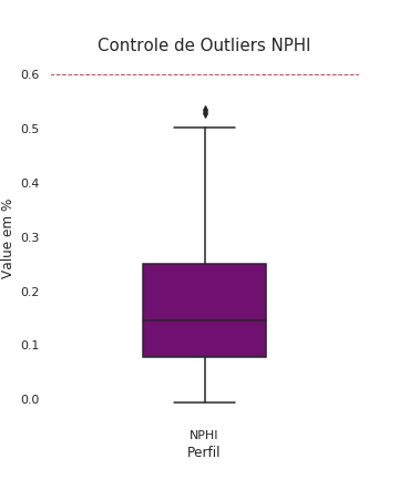
- NPHI varia entre 0 e 60
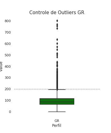
- GR varia entre 0 e 200
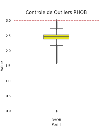
- RHOB varia entre 1 e 3
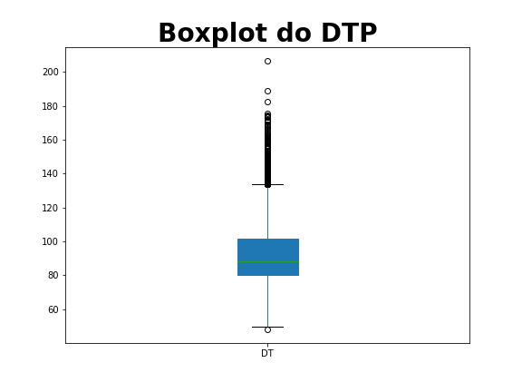
- DT varia entre 0 e 140
graph=sns.boxplot(x=df1['LOG'], y=df1['VALUE'],color='orange',width=0.4)

graph.axhline(140,linewidth=1, linestyle='--',color='r')

plt.xlabel("Perfil", fontsize= 12)
plt.ylabel("Value", fontsize= 12)


plt.title("Controle de Outliers DT", fontsize= 15)
sns.set(rc={'figure.figsize':(5,6)})

plt.savefig('boxplot_dtp_com_outliers.png', transparent = True)
graph=sns.boxplot(x=df2['LOG'], y=df2['VALUE'], color='green',width=0.4)

graph.axhline(200,linewidth=1, linestyle='--',color='r')

plt.xlabel("Perfil", fontsize= 12)
plt.ylabel("Value", fontsize= 12)

plt.title("Controle de Outliers GR", fontsize= 15)

sns.set(rc={'figure.figsize':(5,6)})

plt.savefig('boxplot_gr_com_outliers.png', transparent = True)
graph=sns.boxplot(x=df3['LOG'], y=df3['VALUE'], color='purple',width=0.4)
graph.axhline(.60,linewidth=1, linestyle='--',color='r')

plt.xlabel("Perfil", fontsize= 12)
plt.ylabel("Value em %", fontsize= 12)

plt.title("Controle de Outliers NPHI", fontsize= 15)

sns.set(rc={'figure.figsize':(5,6)})

plt.savefig('boxplot_nphi_com_outliers.png', transparent = True)
graph=sns.boxplot(x=df4['LOG'], y=df4['VALUE'], color='yellow',width=0.3)

graph.axhline(3,linewidth=1, linestyle='--',color='r')
graph.axhline(1,linewidth=1, linestyle='--',color='r')

plt.xlabel("Perfil", fontsize= 12)
plt.ylabel("Value", fontsize= 12)
sns.set(rc={'figure.figsize':(5,6)})

plt.title("Controle de Outliers RHOB", fontsize= 15)
plt.savefig('boxplot_rhob_com_outliers.png', transparent = True)